Automate Change Point Detection in Time Series with Piecewise Regression

A practical grid search approach for detecting trend changes in time series data

Many traditional statistical methods for time series analysis are simple and powerful—but they don’t scale well when applied to large collections of time series. In the previous tutorial, we introduced piecewise regression—a flexible and interpretable approach for modeling time series with underlying trend change points.

The example used in that tutorial—the number of natural gas consumers in California—was intentionally simple. The change point is visually apparent, making it a good teaching example. In real-world scenarios, however, trend changes are often subtle, noisy, or numerous, and identifying them visually is neither reliable nor practical. This becomes especially problematic when working with dozens or hundreds of time series.

Figure 1: Identify the optimal number of knots and their positions using grid search

To address this, we need a programmatic way to identify change points. This is where optimization methods come into play. While there are multiple approaches for estimating trend change points, this tutorial focuses on a grid search strategy combined with piecewise regression to automatically identify the optimal number of change points and their positions.

The full code for this tutorial is available in both R and Python, and a Streamlit app is available here.

Using Grid Search to Find Change Points

Grid search is a simple and systematic optimization technique. It works by evaluating a model over a predefined, discrete set of candidate parameters and selecting the configuration that performs best according to a chosen criterion.

In the context of piecewise regression, these parameters correspond to the number of knots and their positions, which represent candidate change points in the trend.

At a high level, the grid search follows this workflow:

• Define parameters

• Define a cost function

• Fit a piecewise regression for each set of grid combinations

• Score the results

• Select the grid combinations that achieved the optimal results

To reduce overfitting and improve stability, we also enforce a minimum distance between knots, preventing change points from being unrealistically close.

Defining Cost Function

Before running the grid search, we need a way to compare models with different numbers of change points. A cost function (also called a loss function or objective function) is a mathematical function that quantifies how well a model fits the data. It maps a set of model parameters to a single numerical value that represents model error or overall quality.

In machine learning and statistical modeling, the goal of training or model selection is to find the parameter set that minimizes (or maximizes) the cost function.

In regression problems, cost functions typically measure how far the model’s predictions are from the observed data. Common examples include:

• Mean Squared Error (MSE) – measures the average squared residuals

• Mean Absolute Error (MAE) – measures the average absolute residuals

• Negative Log-Likelihood (NLL) – measures how likely the observed data are under the model

While these metrics focus on goodness-of-fit, they do not account for model complexity. As a result, more flexible models—such as piecewise regression models with many change points—will almost always achieve lower error, even when fitting noise.

To address this, we use penalized cost functions that balance fit quality with model complexity. Two widely used examples are the Akaike Information Criterion (AIC) and the Bayesian Information Criterion (BIC). Both are based on the negative log-likelihood but include an explicit penalty for the number of estimated parameters.

Akaike Information Criterion (AIC):

\(AIC=−2log?(L)+2k\text{AIC} = -2 \log(L) + 2kAIC=−2log(L)+2k\)

BIC (Bayesian Information Criterion):

\(BIC=−2log?(L)+klog?(n)\text{BIC} = -2 \log(L) + k \log(n)BIC=−2log(L)+klog(n)\)

Where:

• L = maximized likelihood

• k = number of estimated parameters

• n = number of observations

By penalizing unnecessary complexity, AIC and BIC help prevent overfitting and enable selecting a meaningful number of change points during grid search. Intuitively, BIC penalizes model complexity more strongly than AIC, making it more conservative when selecting the number of change points.

Grid Search Workflow

After laying the foundation, we can define the grid search functionality. A typical grid search procedure for change point detection consists of the following components:

• Prepare the data and define the search space

• Fit a piecewise regression model for a given knot configuration

• Evaluate each configuration using a penalized cost function

• Select the optimal number of knots and their locations

The inputs to such a function are the time series and the search space arguments, and the output is the optimal set of knots.

Figure 3: A general grid search function workflow

One of the main advantages of grid search is its simplicity and ease of implementation. However, this approach can be computationally expensive, especially as the number of candidate change points increases. To address this, we introduce search-space constraints that reduce the number of configurations to be evaluated while improving model stability and interpretability.

In addition to improving computational efficiency, these constraints act as guardrails against overfitting:

• Excluding a fixed proportion of observations at the beginning and end of the series from the change point search, ensuring that each segment contains enough data to support reliable trend estimation

• Enforcing a minimum number of observations per segment, which stabilizes slope estimates and prevents the model from fitting short, noisy segments (e.g., overfitting)

• The maximum number of knots, which defines the possible range of knots per search, and prevents overfitting

There are several factors to consider when setting those parameters, such as the number of observations, the frequency of the series, and business logic.

Note that we use a simple trend model (e.g., with no knots) to benchmark the grid results.

Grid Search Implementation

Let’s go back to the example we used in the previous tutorial - the number of natural gas consumers in California (e.g., the series), and see the implementation of a grid search function with R. A Python version is available in this notebook.

Let’s start with loading the required libraries:

library(dplyr)
library(tsibble)
library(plotly)

In addition, we will source a set of supporting functions from the newsletter repo, including the grid search function - piecewise_regression:

fun_path <- “https://raw.githubusercontent.com/RamiKrispin/the-forecaster/refs/heads/main/functions.R”

source(fun_path)

Next, we will load the series and reformat it:

path <- "https://raw.githubusercontent.com/RamiKrispin/the-forecaster/refs/heads/main/data/ca_natural_gas_consumers.csv"

ts <- read.csv(path) |>
    arrange(index) |>
    filter(index > 1986) |>
    as_tsibble(index = "index")

ts |> head()

This series is yearly, where the index and y columns represent the series timestamp and values:

# A tsibble: 6 x 2 [1Y]
  index       y
  <int>   <int>
1  1987 7904858
2  1988 8113034
3  1989 8313776
4  1990 8497848
5  1991 8634774
6  1992 8680613 

Let’s plot the series:

p <- plot_ly(data = ts) |>
  add_lines(x = ~ index,
            y = ~ y, name = "Actual") |>
            layout(
        title = "Number of Natural Gas Consumers in California",
        yaxis = list(title = "Number of Consumers"),
        xaxis = list(title = "Source: US energy information administration"),
        legend = list(x = legend_x, y = legend_y)
    )

p

Figure 4: Yearly number of natural gas consumers in California. The series is trending up without seasonality patterns

Let’s use the grid search function - piecewise_regression to identify the optimal number of knots and their positions:

grid <- piecewise_regression(
    data = ts,
    time_col = "index",
    value_col = "y",
    max_knots = 4,
    min_segment_length = 8,
    edge_buffer = 0.05,
    grid_resolution = 20
)

We use the following arguments to define the search space:

• max_knots - the maximum number of knots

• min_segment_length - the minimum number of observations between two knots

• edge_buffer - the percentage of observations to exclude from the tail and head of the series

• grid_resolution - the maximum number of search combinations per number of knots

We set the max_knots argument to 4, limiting the possible number of knots in the search space to 0-4. The function creates the search space according to the above constraints and trims options that do not meet them.

This returns the following output:

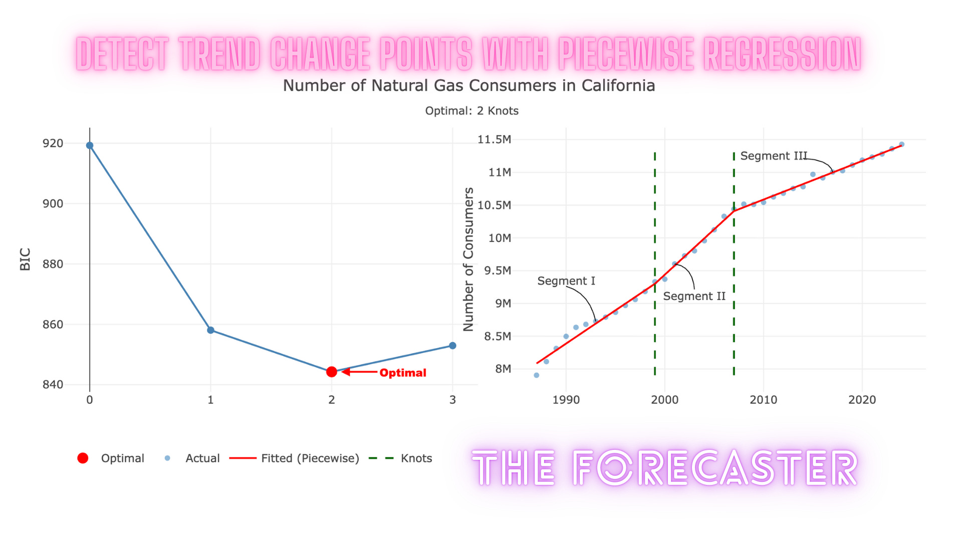
Testing 0 knot(s)...
  Best BIC: 919.28 | RSS: 1.006639e+12 | Tested 1 configurations
Testing 1 knot(s)...
  Best BIC: 858.05 | RSS: 182625404855 | Tested 18 configurations
Testing 2 knot(s)...
  Best BIC: 844.26 | RSS: 115452860424 | Tested 25 configurations
Testing 3 knot(s)...
  Best BIC: 852.94 | RSS: 131838198802 | Tested 5 configurations
Testing 4 knot(s)...

Optimal model:  2 knot(s) with BIC = 844.26 
Warning message:
In generate_candidates(k, min_idx, max_idx, min_segment_length) :
  Cannot fit 4 knots with min segment length 8

Which includes the number of tested models by the number of knots and the optimal number of knots - 2. In addition, you can see that the function returned a warning that it did not fit models with 4 knots because it lacked a sufficient number of observations due to the search space constraints. This is expected behavior and indicates that the search space constraints are working as intended.

The animation below illustrates the fit of all the search space options:

Figure 5: Animation of the grid search process

The output of the function includes information about the search and the optimal number of points, such as the optimal number of knots:

grid$optimal_knots
[1] 2

And their positions:

grid$knot_dates
[1] 1999 2007

Last but not least, we will use the plot_knots function and add some annotations to plot the series with the optimal points:

Figure 6: The optimal number of knots and their positions based on the grid search results

When This Change Point Detection Method May Not Work Well

As demonstrated in this tutorial, using grid search with piecewise regression is an effective way to identify the optimal number and location of trend change points. This approach performs best on relatively “clean” time series where the dominant signal is the underlying trend, as in the example used here.

In practice, however, many real-world time series also contain additional patterns—such as seasonality, abrupt level shifts, or outliers—that can obscure or distort the trend component. When these effects are present, the grid search may identify spurious change points or fail to recover meaningful trend breaks.

In such cases, it is often beneficial to first apply a decomposition method to isolate the trend component (e.g., via STL or similar techniques), and then perform the grid search on the extracted trend rather than on the raw series.

Alternatively, more advanced change-point detection methods that jointly model trend and seasonality may be more appropriate for highly structured or noisy series.

Summary

In this tutorial, we demonstrated how to automatically detect trend change points in time series data using a grid search strategy combined with piecewise regression. By framing change-point detection as an optimization problem, we systematically evaluated candidate knot configurations and selected the optimal model using a penalized likelihood criterion.

Key takeaways include:

• Piecewise regression provides an interpretable framework for modeling trend changes

• Grid search offers a simple yet effective approach for estimating change point locations

• Penalized criteria, such as BIC, balance goodness-of-fit with model complexity and help prevent overfitting

• Search-space constraints (edge buffers, minimum segment length, and maximum knots) improve model stability and computational efficiency

While grid search is not the most computationally efficient approach, its transparency makes it an excellent baseline and a practical solution for many real-world applications. In more complex settings, this framework can be extended using advanced optimization or Bayesian change-point detection methods. In the next tutorial, we will review how to apply this method to more complex scenarios.

Resources

• Introduction to Piecewise Regression

• The code used in this tutorial is available in both R and Python

• A Streamlit app illustrates this method