
Piecewise Regression for Time Series Forecasting
Modeling a Trend Change Point with Feature Engineering Approach

Modeling trends is a fundamental part of time series analysis and forecasting. In many real-world time series, however, the underlying trend does not remain constant. Instead, the series may exhibit trend changes, also known as change points or structural breaks, in which the slope of the trend shifts due to external or systemic factors.
If these change points are not modeled explicitly, forecasting models—especially simple regression-based models—can suffer from biased estimates and increasing forecast errors. This is particularly problematic when the trend dominates the series's behavior, as is often the case in long-term forecasts.
Piecewise regression, also referred to as piecewise linear regression or segmented regression, provides a simple and effective way to model such trend changes. Rather than relying on a single global trend, piecewise regression allows the trend to change at predefined time points by introducing additional, carefully designed features. From a practical perspective, this approach can be viewed as a feature engineering technique for handling change points in time series data.
In this tutorial, we introduce the core idea behind piecewise regression and show how it can be used to model trend change points in a time series. We begin by fitting a simple linear trend model, demonstrate why it fails in the presence of a change point, and then show how adding knot-based features enables the model to capture multiple trend regimes. For clarity and interpretability, we use linear regression in the examples, but the same approach applies to other regression models, such as Ridge, Lasso, XGBoost, or k-nearest neighbors. The full code for this tutorial is available in both R and Python.
Modeling Trend with Simple Linear Trend
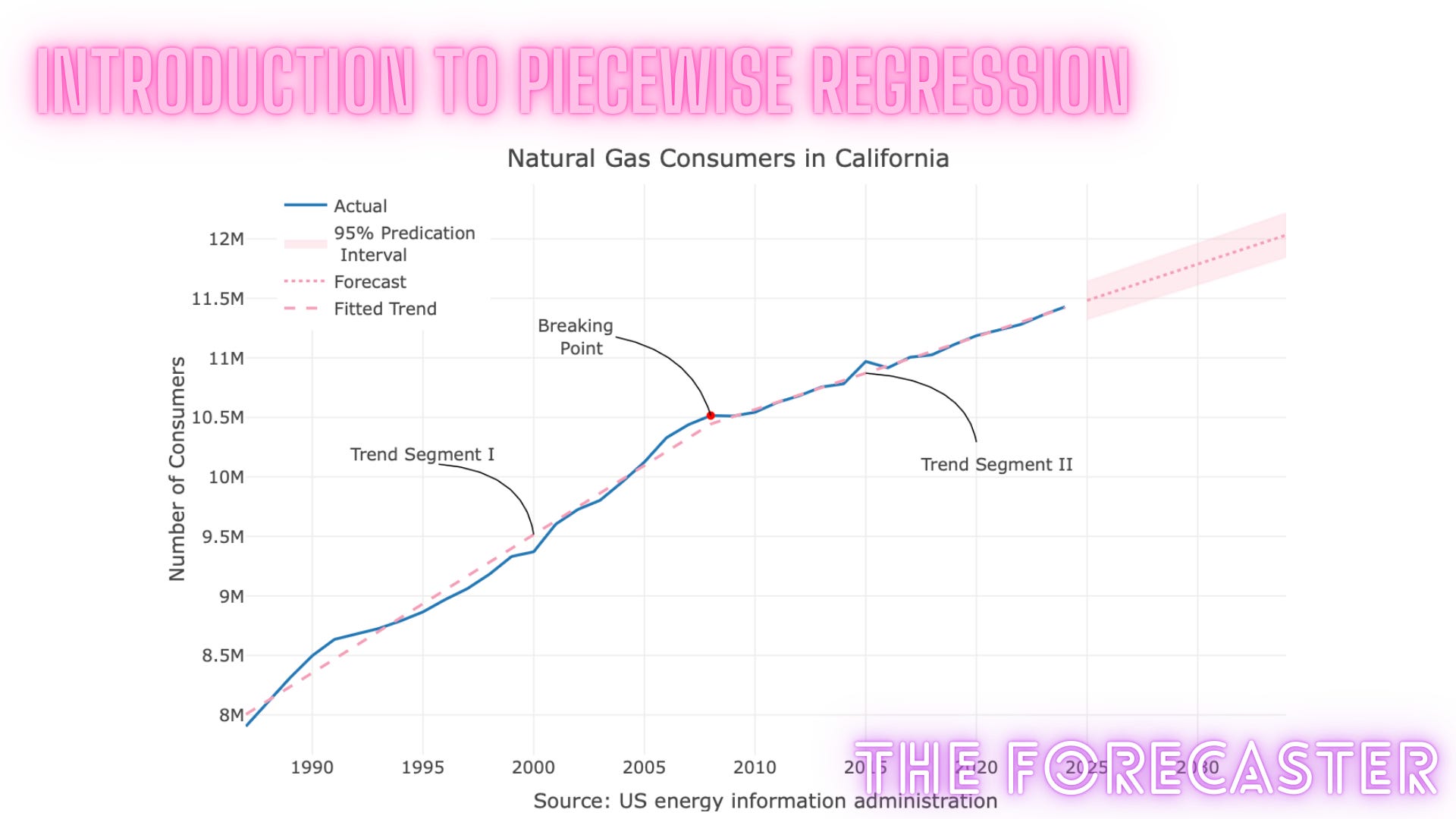
To understand how piecewise regression works, we will use the number of natural gas consumers in California. This yearly series, as shown in the figure below, is fairly simple, with no seasonality and little fluctuation. This will enable us to focus on the piecewise regression method without worrying too much about other patterns.

The main things that pop up after eyeballing the series:
The series has no seasonality
It trending up
There is a change in the trend (or a change point) around 2008
Before we dive into more details about piecewise regression and how we will handle the trend change point, let’s build a baseline forecasting model using a simple linear trend. This simply means that we will regress the series against an arbitrage index using the following simple regression formula:
Where Y represents the series, and Index is simply a vector of arbitrage numbers that increase as a function of time:
Using a linear regression model will give us the following results:

The intuition behind this approach is that, using regression, we calculate the average change in the series for each time step. Or in simple words, the trend coefficient represents the series growth under the assumption that the growth is linear. For the number of natural gas customers in California, the trend coefficient implies that the number of customers is growing by about 94,000 per year on average.
Without going into whether this number is accurate, that is the general mathematical notion when modeling a time series trend with a regression model.
While this method is effective when there is a linear trend, it is sensitive to changes in the trend. To better understand this, let’s add the regression line to the series plot and assess the model’s goodness-of-fit.

As you can see from the above plot, as we progress in time towards the end of the series, the fitted values are gradually overestimate the true value of the series. The main reason that the model cannot handle this case well is related to the properties of the simple linear regression:
It is a weighted average
It must pass through the interception of the averages of the y and x dimensions
Those constraints make the model have a “hard time” fitting a linear trend when change points are present in the series.
In many cases, the impact of the series trend on model accuracy is significantly greater than that of other features, such as outliers and seasonality. If we try to forecast this series, you can notice that, under the assumption that the recent trend of the series will remain the same, your forecast error rate will increase as a function of the forecast horizon:

Modeling Trend with Change Points with Piecewise Regression
After laying the foundation and seeing why simple linear regression fails to model a series with trend changes, we are ready to introduce piecewise regression. I found the term “Piecewise Regression” a bit misleading, as it is not necessarily a regression method, but rather a feature engineering approach. As we saw above, we use an index feature (named as trend) to model the marginal change of one unit of time. When a series has break points in the trend, we simply add a knot at each break point. A knot feature enables us to inform the model of a change in the trend slope. From a feature engineering perspective, if similar to the trend feature, with the exception of:
Left to the knot point - equals zero
From the knot point to the right - an arbitrage numbers that increase as a function of time
Therefore, it enables the regression model to split the trend into two segments (when using a single knot) - before and after the change point. Of course, you can have more than one knot, where each point introduces a new state of the series trend to the model.
For example, let’s assume we want to add a knot to the series at point c, we then add a second feature to the previous regression named as knot:
The knot feature is defined, with respect to t and c:
Where t represents the series timestamp, and c represents the knot timestamp. Whereas before, the trend feature is an index vector:
The following figure illustrates how those features vary with respect to the series:

Let’s add to the previous model knot in 2008, and set the knot feature accordingly (e.g., c = 2008), run the regression model, and evaluate the results:

The nice thing about model coefficients, particularly in a linear regression model, is their straightforward interpretability. As shown in the regression table above, the knot feature is negative, indicating an offset to the series’ initial trend, starting at point c. This split the trend into two segments, enabling us to have a better fit of the trend, as can be seen in Figure 5:

While this model still uses a linear trend, it accounts for a change in slope in the series that occurred approximately in 2008. Last but not least, we can reforecast the series with the new model:

That forecast looks much better!
Summary
In this tutorial, we introduced piecewise regression, a powerful yet intuitive method for modeling change points in time series trends. By augmenting a standard regression model with knot-based features, piecewise regression allows the trend slope to change at specific points in time while maintaining the simplicity and interpretability of linear models.
This approach effectively splits a single global trend into multiple linear segments, making it well suited for time series with structural breaks or evolving growth patterns. Piecewise regression is especially useful in forecasting applications, where unmodeled trend changes can lead to rapidly increasing forecast errors as the horizon extends.
In the next tutorial, we will explore methods for identifying the optimal number and location of change points, including data-driven and statistical approaches for selecting knot positions.